What is LaTeX?
Overview
Teaching: 10 min
Exercises: 0 minQuestions
What does LaTeX do?
Objectives
Explain what LaTeX is
Explain how it differs from a wordprocessor
What is LaTeX?
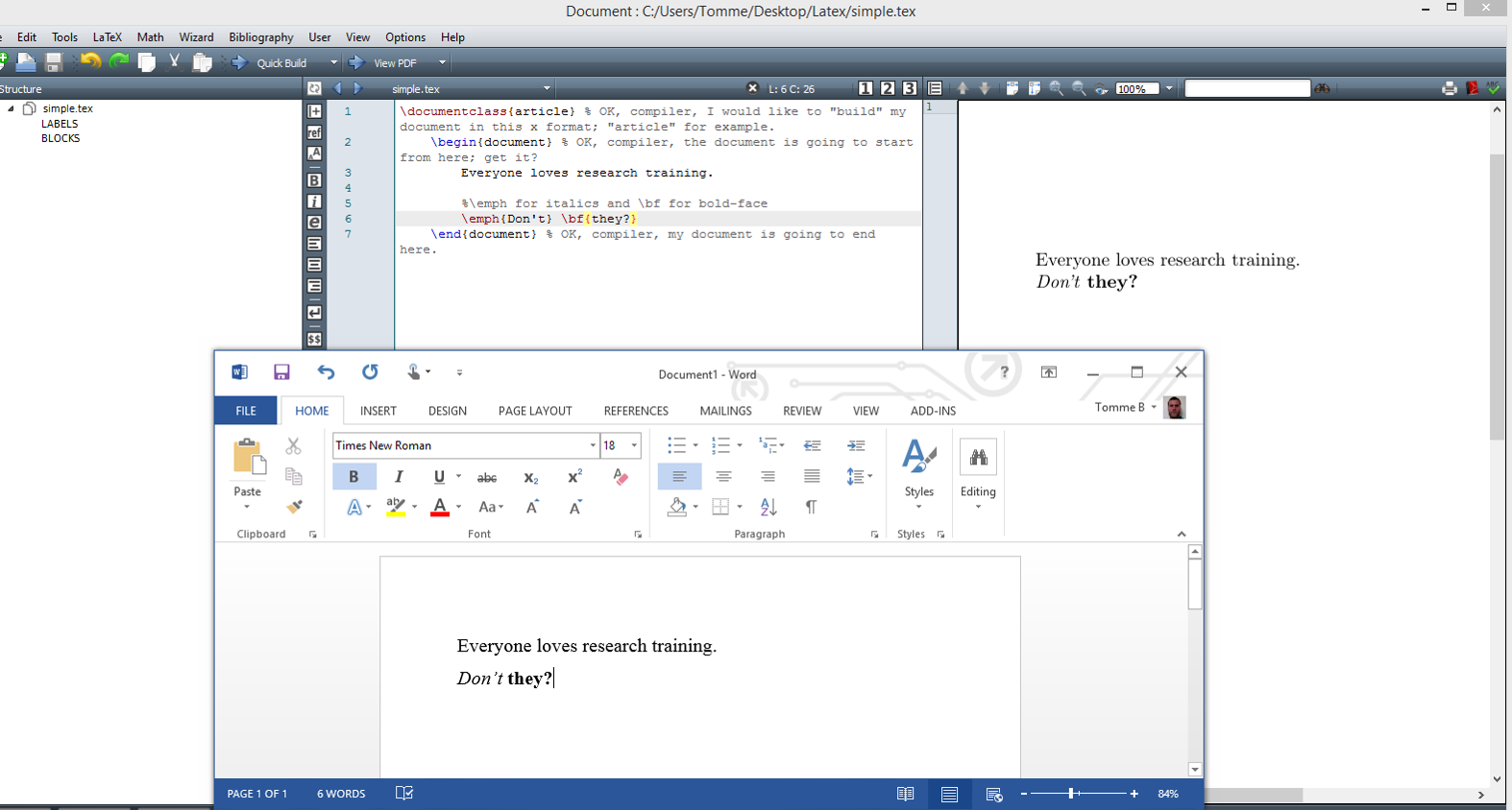
LaTeX (pronounced Laytec) is a document preparation and typesetting system that has been around since the early 1980s. Unlike a traditional word processor such as Microsoft Word or Libreoffice it works by using a markup language and converting this into a document file, typically a PDF. Where exactly things appear on the page is determined by LaTeX itself leaving you to focus on the content of your document. Like with a wordprocessor you can create chapters, sections and subsections, set the style of certain parts of the text, insert citations and cross references, tables, images, equations etc.
Why use it?
- Separates layout and content
- Formatting (mostly) handled automatically
- Good handling of citations and references
- Easy to write maths into a document
- Popular in academic publishing, some journals and conferences will supply a LaTeX template.
- Free and Open Source
- Produces beautiful documents
Why not to use it?
- A bit of an initial learning curve
- Can feel more like computer programming than document writing
- Unhelpful error messages
- Complicated set of addons
- Getting things to look exactly how you want can be hard
- You can’t see exactly what the document will look as you work on it (although some editors have live previews)
LaTeX vs TeX
LaTeX is really a series of macros written in a typesetting language called TeX. These make LaTeX much simpler and easier to use than writing TeX yourself.
Key Points
LaTeX is a document preparation and typesetting system
It uses markup language
Separates style from contents
(Usually) Does a good job of typesetting
Outputs to a PDF or Postscript file
Running LaTeX
Overview
Teaching: 10 min
Exercises: 5 minQuestions
how do we build a LaTex document?
What are the common editors for LaTeX?
Objectives
Explain that LaTeX is compiled
Introduce TexStudio and Overleaf editors
Setting up LaTeX
- Linux users install the package texlive using your package manager and TeXStudio
- Windows users install MiKTeX and TeXStudio
- Mac users download MacTeX and TeXStudio
- If you can’t install anything you can use Overleaf in your web browser.
Running LaTeX from the command line
LaTeX code has to be ‘compiled’ to convert it from the LaTeX language into a PDF file which can be easily viewed, distributed or printed. One method for doing this is to run the command pdflatex from the command line and tell it which LaTeX file we want to compile. Providing there are no errors this will convert the LaTeX into a PDF file.
Download the example file helloworld.tex.
Or type out the code in your favourite text editor and save it as helloworld.tex
\documentclass{article}
\begin{document}
\title{Hello World}
\author{Jane Doe}
\maketitle
\end{document}
pdflatex helloworld.tex
This should produce some output like:
This is pdfTeX, Version 3.14159265-2.6-1.40.18 (TeX Live 2017/Debian) (preloaded format=pdflatex)
 restricted \write18 enabled.
entering extended mode
(./helloworld.tex
LaTeX2e <2017-04-15>
Babel <3.18> and hyphenation patterns for 7 language(s) loaded.
(/usr/share/texlive/texmf-dist/tex/latex/base/article.cls
Document Class: article 2014/09/29 v1.4h Standard LaTeX document class
(/usr/share/texlive/texmf-dist/tex/latex/base/size10.clo)) (./helloworld.aux)
[1{/var/lib/texmf/fonts/map/pdftex/updmap/pdftex.map}] (./helloworld.aux) )</us
r/share/texlive/texmf-dist/fonts/type1/public/amsfonts/cm/cmr10.pfb></usr/share
/texlive/texmf-dist/fonts/type1/public/amsfonts/cm/cmr12.pfb></usr/share/texliv
e/texmf-dist/fonts/type1/public/amsfonts/cm/cmr17.pfb>
Output written on helloworld.pdf (1 page, 26419 bytes).
Transcript written on helloworld.log.
It should also create a file called helloworld.pdf in the same directory which you can open in a PDF viewer such as Adobe Acrobat. It will also create some other temporary files called helloworld.aux and helloworld.log. These can be deleted afer you’ve compiled your document.
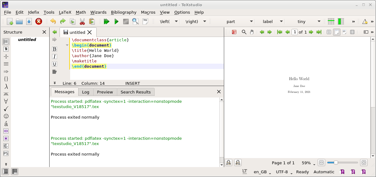
Running LaTeX from TeXstudio
Now we’ll paste the same code we used above into TeXstudio, then save the document and press the green button that looks like a play symbol with a tail on it or press the ‘F5’ key or click on the “Tools” menu and choose “Build and View”.

Building a PDF with TeXstudio
Instead of previewing inside TeXstudio we can also build a PDF file by clicking on the green Play button, pressing ‘F6’ or choosing ‘Compile’ from the Tools menu.
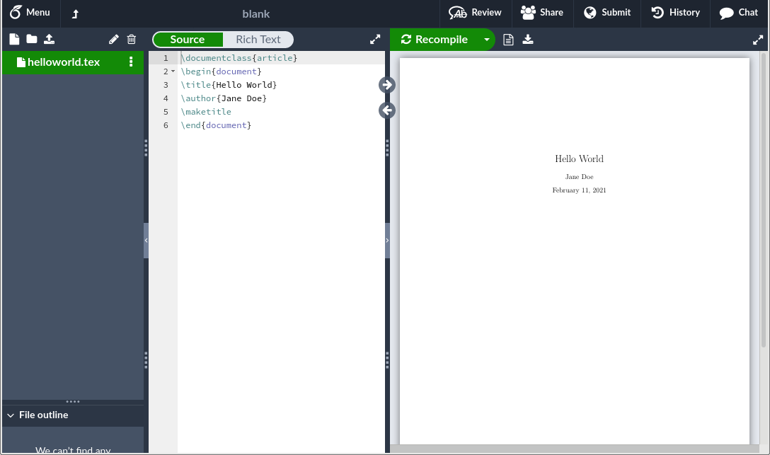
Running LaTeX from Overleaf
- Go to www.overleaf.com in your web browser.
- Create a new account (if you don’t already have one) and login.
- Click on “New Project” and choose “Blank Project”, give the project a name.
- You’ll be taken to a screen with some example LaTeX code already entered.
- Replace this with the code we entered above or upload the
helloworld.texfile we downloaded. - Click on the green “Recompile” button near the top middle of the screen.
- After a few seconds this should build your document and show it on the right side of the screen.
- Click on the download icon if you want a copy of the PDF.
Compiling a document yourself
Pick one of the methods shown above (a simple text editor, TeXStudio or Overleaf) and do the following:
- Paste in the hello world document above.
- Change the author to your own name.
- Compile the code to make a PDF file and open it in a PDF viewer.
Key Points
LaTeX is compiled by running the pdflatex command
There are lots of editors which include a button to run pdflatex
Some editors like Overleaf include a preview of your document
LaTeX Commands
Overview
Teaching: 15 min
Exercises: 10 minQuestions
What are the three different styles of LaTeX command?
Objectives
Understand how LaTeX commands are structured
See the difference between commands that take no arguments, one’s which take an argument and one’s which use a begin and end command.
LaTeX Commands
Commands with no arguments
As you’ve seen from the simple Hello World example, LaTeX commands all start with a ‘' character. We saw three types of examples on the previous page. The simplest was just a slash followed by a command, which was the maketitle command. This command takes some of the information that was already given and displays the title block.
\maketitle
LaTeX has a number of other commands like this, one of the most useful is \newpage which will insert a new page into the document. Lets modify our old document to have an extra page using this command:
\documentclass{article}
\begin{document}
\title{Hello World}
\author{Jane Doe}
\maketitle
\newpage
\end{document}
But when we build this document it still doesn’t have a second page, because LaTeX has decided since there’s no content after the \newpage command it won’t include the page. Lets add some extra text after the \newpage. Now the text ‘hello world’ will appear on the second page (and if we remove the \newpage it will appear on the first page.
\documentclass{article}
\begin{document}
\title{Hello World}
\author{Jane Doe}
\maketitle
\newpage
Hello World
\end{document}
Commands with arguments
Some commands in LaTeX take an argument or some extra information. This is done by writing a { and } symbol after the command and entering the arguments between them. We already saw this in the documentclass, author and title commands. Another useful command that works in this style is the \textbf command. This makes the text that appears between the { and } symbols into bold text. Lets try making the Hello World text we just wrote in bold.
\documentclass{article}
\begin{document}
\title{Hello World}
\author{Jane Doe}
\maketitle
\newpage
\textbf{Hello World}
\end{document}
Environments
Our third type of commands are called environments. They use a \begin and \end statement and span multiple lines, everything in between the begin and end statement is part of the environment. We saw this already with the \begin{document} and \end{document} commands, the content of our entire document should be between these. These state that everything between the begin and end commands are part of the document. Another environment we can use in this way is the abstract environment which uses the \begin{abstract} command, the text for our abstract is then placed between the \begin{abstract} and the \end{abstract}. We can place this anywhere in the code that we like, but we probably want it to appear just after the title and on its own page, so lets take the code we just wrote and add the abstract after the newpage and before the bold hello world. Note that the abstract environment is nested inside the document environment.
\documentclass{article}
\begin{document}
\title{Hello World}
\author{Jane Doe}
\maketitle
\newpage
\begin{abstract}
The text for my abstract..
\end{abstract}
\textbf{Hello World}
\end{document}
This now puts the abstract and the bold Hello World on the same page, perhaps this isn’t quite what we want so lets add another page between them:
\documentclass{article}
\begin{document}
\title{Hello World}
\author{Jane Doe}
\maketitle
\newpage
\begin{abstract}
The text for my abstract..
\end{abstract}
\newpage
\textbf{Hello World}
\end{document}
Using the \bigskip command
The command \bigskip creates a big empty section between two bits of text. Add a \bigskip to this document, after the abstract ends but before the document text.
\documentclass{article}
\begin{document}
\title{Hello World}
\author{Jane Doe}
\maketitle
\newpage
\begin{abstract}
The text for my abstract..
\end{abstract}
The document text
\end{document}
Solution
\documentclass{article}
\begin{document}
\title{Hello World}
\author{Jane Doe}
\maketitle
\newpage
\begin{abstract}
The text for my abstract..
\end{abstract}
\bigskip
The document text
\end{document}
Using the \textit command
The \textit command makes the text contained between its { and } characters into italics. Try using this command to make some italic text in your document.
Solution
\documentclass{article}
\begin{document}
\title{Hello World}
\author{Jane Doe}
\maketitle
\newpage
\begin{abstract}
The text for my abstract..
\end{abstract}
\textit{The document text}
\end{document}
Centering Text
The
\begin{center}command will centre all text that follows it until a\end{center}command is issued. Try using this command to centre the text in your document.Solution
\documentclass{article}
\begin{document}
\title{Hello World}
\author{Jane Doe}
\maketitle
\newpage
\begin{abstract}
The text for my abstract..
\end{abstract}
\begin{center}
The document text
\end{center}
\end{document}
Key Points
LaTeX uses a series of commands all beginning with a \ character
Some commands take additional arguments between a { and } character
Some commands, known as environments lots of additional content between begin and end commands
Structuring LaTeX Documents
Overview
Teaching: 15 min
Exercises: 5 minQuestions
How do you break up the structure of a LaTeX document?
Objectives
Explain about the different sections of a document
Structuring LaTeX Documents
We’ve already seen that documents can have abstracts as a part of the document, but they can also have many other types of section to split up the document. We can declare sections, subsections, subsubsections and paragraphs using the commands: \section{title}, \subsection{title}, \subsubsection{title} and \paragraph{title}.
\documentclass{article}
\begin{document}
\title{My first LaTeX paper}
\author{Jane Doe}
\maketitle
\newpage
\section{Introduction}
Write introduction here....
\section{Background}
Write background here...
\section{Methods}
Write methods here...
\section{Results}
Write results here...
\section{Conclusion}
Write conclusion here...
\end{document}
After compiling this document you should see that each section now has a bold heading with larger text and is numbered from 1 to 5. This numbering is automatic, if we change the order, add or remove a section the numbers will automatically change. Now lets add a table of contents by using the command \tableofcontents under the \maketitle line. Now on the first page there should be a title and a table of contents and on page two we’ll have the sections and their contents.
\documentclass{article}
\begin{document}
\title{My first LaTeX paper}
\author{Jane Doe}
\maketitle
\tableofcontents
\newpage
\section{Introduction}
Write introduction here....
\section{Background}
Write background here...
\section{Methods}
Write methods here...
\section{Results}
Write results here...
\section{Conclusion}
Write conclusion here...
\end{document}
Creating subsections and subsubsections.
Take the document above and add a subsection on Future Work to the conclusion and a subsubsection on exciting things I didn’t have time for under the future work subsection.
Solution
\documentclass{article}
\begin{document}
\title{My first LaTeX paper}
\author{Jane Doe}
\maketitle
\tableofcontents
\newpage
\section{Introduction}
Write introduction here....
\section{Background}
Write background here...
\section{Methods}
Write methods here...
\section{Results}
Write results here...
\section{Conclusion}
Write conclusion here...
\subsection{Future Work}
Write about future work here.
\subsubsection{Really Exciting Thing I didn't have time for}
Write about the really exiciting thing here.
\end{document}
Creating Chapters
Try putting all your sections inside a chapter by using the
\chapter{title}command before the first section. Does this work? If not what error does it produce and why? How might you fix this?Solution
You will get an error message saying “Undefined control sequence \chapter”. This is because chapter isn’t supported by the article document class since articles don’t usually have chapters. If you change the document class from article to report then it should allow chapters.
Adding Appendicies
To add Appendicies on the end of a document we need to first use a class that supports them. The report class is one example of a document class which supports them. Each appendix is really just a chapter, but LaTeX will start calling them Appendix instead of Chapter after we issue the command \appendix. For example:
\documentclass{report}
\begin{document}
	\title{My first LaTeX paper}
	\author{Jane Doe}
	\maketitle
	\newpage
	\tableofcontents
	\newpage
	\chapter{My Chapter}
	\section{Introduction}
	Write introduction here....
	\section{Background}
	Write background here...
	\section{Methods}
	Write methods here...
	\section{Results}
	Write results here...
	\section{Conclusion}
	Write conclusion here...
	\subsection{Future work}
	Write about what you'll do in future.
	\subsubsection{Thing I'm really exited about}
	There's this thing I didn't have time for that might be really exciting.
	\paragraph{Why its so it exciting}
	Because its so good!
	\appendix
	\chapter{Stuff I couldn't fit}
		Write appendix here
\end{document}
Sometimes you have to recompile multiple times
Sometimes things such as table of contents don’t update the first time we recompile a document after adding them. This is because some information about things further into the LaTeX document isn’t known the first time we compile, but as it compiles its entered into the .aux file which is read by the LaTeX compiler on the second pass. As we’ll see in a future section the same thing can happen with bibliographic references.
Labelling and Referencing Sections
It can be useful to be able to reference another section by its number of a document sometimes, for example to be able to say “see section 5 for more discussion about this”. LaTeX can help us do this and automatically keep the section number correct even as we make changes to the document. To do this we need to do two things, firstly we have to label the section being referred to and then we have to reference that label. This is done with the \label{} and \ref{} commands. The label command wants us to give the label a name, by convention if we’re labelling a section we’ll start the label with “sec:”, a subsection with “subsec:”. As we’ll see later labels can also be used for figures and tables and these would start their labels “fig:” or “tab:”. This is only a convention though and LaTeX doesn’t actually care what you use, but when you create a large document with hundreds of labels it can really help to know which is which.
\documentclass{article}
\begin{document}
	\title{My first LaTeX paper}
	\author{Jane Doe}
	\maketitle
	\newpage
	\tableofcontents
	\newpage
	\section{Introduction}
	Write introduction here....
	\section{Background}\label{sec:background}
	Write background here...
	\section{Methods}
	As we discussed in section \ref{sec:background}......
\end{document}
When it compiles you should see that \ref{sec:background} is replaced with “2”. If we were now to insert another section between Introduction and Background it would automatically change to “3”.
Key Points
LaTeX lets us split up documents into sections, subsections, subsubsections etc.
Some document classes allow extra commands like chapters, tables of contents etc.
We can label parts of the document with the label command and reference them with the \ref{} command
Styling Documents and Lists
Overview
Teaching: 15 min
Exercises: 5 minQuestions
How do style the text in LaTeX documents?
How can we create lists in LaTeX?
Objectives
Understand how to apply styles to LaTeX documents
Styling Text
We already saw the \textbf{} command for bold text and \textit{} command for Italic text. But LaTeX offers a few other text styling commands including \underline{} command for underlined text, \textsubscript{} for subscript and \textsuperscript{} for superscript text.
Setting Text Sizes
Text size can be adjusted by using the commands \tiny, \small, \normalsize, \large and \huge. These will set the size of the text until another size command is issued. They also don’t create a new lines, so you can have multiple sizes of text on the same line.
\documentclass{article}
\begin{document}
	\section{Introduction}
	\tiny
	tiny text
	\small
	small text
	\normalsize
	normal text
	\large
	big text
	\huge
	huge text
\end{document}
Special Characters
Some characters which we can type on the keyboard won’t actually appear if we type them into a LaTeX document. Perhaps the best example of this is the ‘%’ character which means a comment in LaTeX. To insert this into a document we need to use the \% command. There are many other symbols which need LaTeX commands, including the £ symbol (\textsterling or \pounds), the less than and greater than symbols (\textless and \textgrater). See this webpage from Wikibooks for a list of common symbols. Note that Overleaf is smarter than other LaTeX distributions and will accept some special characters like the £ symbol, but these documents will not compile correctly on other LaTeX distributions and you should use the correct commands instead of the symbols.
Symbols exercise
Write a letter in LaTeX saying the following: Dear Professor Schrödinger, Please find enclosed €200 for the cat you sold me. Yours Sincerely Émilie du Châtelet
Solution
\documentclass{letter}
\usepackage{eurosym}
\begin{document}
Dear Professor Schr\"odinger,
Please find enclosed \euro{200} for the cat you sold me.
Yours Sincerely \'Emilie du Ch\^atelet
\end{document}
LaTeX Packages
The \usepackage{} command is used to include extra packages, which is sometimes needed for extra symbols (and other extra commands and functionality to LaTeX). You will have needed to use this in the previous exercise to load the Euro symbol. This command is typically placed betwen the \documentclass{} and \begin{document} lines of a LaTeX file. One useful package is the siunitx package which includes SI units for many measurements. Sometimes you might also additional arguments to the package given between [ and ] symbols between the end of the package name and the { character.
\documentclass{article}
\usepackage{siunitx}
\begin{document}
The car was speeding at \SI{150}{\metre\per\second}.
\end{document}
This will display the speed as km h to the power -1. We’re probably more used to seeing km/h, we can set this by adding the command \sisetup{per-mode=symbol} after the \usepackage line.
Whitespace Characters
Putting in multiple spaces or blank lines into our LaTeX source will still only result in one space or newline appearing in the output. Even if we end a line at what we think is a logical place and put in a newline, LaTeX won’t create one there. If we really want extra spaces we have to use \space or for a newline its \newline.
Lists
There are two types of lists which LaTeX can create, numbered lists and un-numbered lists. A numbered list is created with the \begin{enumerate} command, while un-numbered lists are created with the \begin{itemize} command.
\documentclass{article}
\begin{document}
\begin{itemize}
   \item First Item
   \item Second Item
\end{itemize}
\end{document}
Its also possible to nest one list inside another, even if that list is of a different type.
\documentclass{article}
\begin{document}
\begin{itemize}
   \item First Item
   \begin{enumerate}
      \item first numbered item
    \end{enumerate}
\end{itemize}
\end{document}
Lists and packages exercises
- Replace the _____ sections with the correct answers.
- What does \sisetup{group-separator = {,}} do on the third line?
- What happens if you change the group-separator to a dot (.) symbol? Note: newer versions of the siunitx package do not need the [binary-units=true] modifier, this enabled siunitx to handle bytes as a unit.
\documentclass{article}
\usepackage[binary-units=true]{siunitx}
\sisetup{group-separator = {,}}
\begin{document}
 \begin{itemize}
     \item \SI{1}{\tera\byte} (terabyte) is equivalent to:
     \begin{_________}
         \item \SI{1024}{\___\byte} (gigabytes)
         \item \SI{1048576}{\___\byte} (megabytes)
         \item \SI{1099511627776}{\kilo\byte} (kilobytes)
         \item \SI{1208925819614629174706176}{\byte} (bytes)
     \end{enumerate}
 \end{itemize}
\end{document}
Solution
- enumerate, giga and mega.
- Makes the separator between each 3 digits a comma instead of the default space.
Autorecognising Symbols
The website “Detexify” allows you to draw a symbol with your mouse (or finger/pen if you’re using a phone or tablet) and will attempt to recognise it and tell you the LaTeX symbol for it.
Key Points
We can style text with bold, underline, italic, superscript etc
Some characters such as accented characters, £ signs, percent signs need special LaTeX commands to appear.
Extra spaces don’t get shown by LaTeX, use the space command if you want extra spaces or newline to get a newline
Some extra characters can be added by using some extra packages. The Siunitx is one such package, it provides SI units.
We can make numbered lists with the enumerate environment.
We can make un-numbered lists with the itemize environment.
Figues and Tables
Overview
Teaching: 15 min
Exercises: 15 minQuestions
How do you create tables in LaTeX?
How do you insert images in LaTeX?
Objectives
Understand how to create tables
Understand how to insert images
Understand that LaTeX tries to determine where to place images and tables but doesn’t always get this right.
Understand how to override the placement options
Tables in LaTeX
Table Headings
Tables in LaTeX are probably one of the “less nice” bits of the language and can be a little fiddly to get working. They are created using the \begin{tabular} and \end{tabular} commands. Each column’s justification is then specified with a single letter, l for left, c for centre or r for right. You need to put one letter for each column you want to create.
\begin{tabular}{ l l l}
The above will create a table with 3 columns that are all left justified.
Custom Column Widths
You can also specify a custom with column with the p column type, folow this with {1cm} to have a 1 centimetre wide column.
\begin{tabular}{ p{1cm} p{1cm} p{1cm}}
Table Contents
Now we need to specify the contents of a table. This is done by writing the value for a column, then an & symbol to get the next colmun and finally ending the line with a \\. For example:
1 & 2 & 3 \\
will create put 1, 2, 3 into the first, second and third columns. We can then repeat this process for as many rows as we want.
Ending the table
To end the table we used the \end{tabular} command.
Putting a line between each column/row
Placing a | symbol between each column heading specification will show vertical lines down the table. If we want a line between rows we can use the \hline command at the end of the rows (it doesn’t have to be on every row).
\begin{tabular}{l | l | l}
\hline
1 & 2 & 3 \\ \hline
4 & 5 & 6 \\ \hline
7 & 8 & 9 \\ \hline
\end{tabular}
Centering the entire table
Its quite common to see entire tables placed inside center blocks (starting with \begin{center} and ending with \end{center}). This centers the entire table on the page. For example:
\begin{center}
\begin{tabular}{l | l | l}
\hline
1 & 2 & 3 \\ \hline
4 & 5 & 6 \\ \hline
7 & 8 & 9 \\ \hline
\end{tabular}
\end{center}
Captioning and Labelling Tables
A can be captioned with the \caption{} command, but before we can use this we have to wrap the table inside an extra container using the \begin{table} and \end{table} commands wrapping the entire table. For example:
\begin{table}
\begin{center}
\begin{tabular}{l | l | l}
\hline
1 & 2 & 3 \\ \hline
4 & 5 & 6 \\ \hline
7 & 8 & 9 \\ \hline
\end{tabular}
\end{center}
\caption{A table}
\end{table}
This table environment also automatically numbers the tables in the order they appear in the document.
Labelling Tables
We saw the \label{} command back when we were talking about sections of a document. We can use it with a table too, so that we can reference the table’s number elsewhere in a document with the \ref{} command. By convention labels for tables will be started with the word tab:, but LaTeX doesn’t enforce this.
\begin{table}
\begin{center}
\begin{tabular}{l | l | l}
\hline
1 & 2 & 3 \\ \hline
4 & 5 & 6 \\ \hline
7 & 8 & 9 \\ \hline
\end{tabular}
\end{center}
\caption{\label{tab:example}A table}
\end{center}
\end{table}
See table \ref{tab:example} for a table of numbers.
An Easy Table Generator
Tables exercise
Create a table to show a calendar and do the following:
- Give it 7 columns and 5 rows,
- Make each 1.5cm wide
- Make the first row the days of the week, starting from Monday (or just Mon). Make these in bold text.
- Put a 1 in the first column on the second row and work up to 28. This should give a calendar for February 2021.
- Create a solid line between the days of the week and the numbers
- Caption it “Calendar for February 2021”
- Give it the label “tab:calendar-feb-2021”, write some text to reference this label underneath the table.
Solution
\documentclass{article}
\begin{document}
\begin{table}
	\begin{center}
	\begin{tabular}{p{1.5cm}  p{1.5cm}  p{1.5cm}  p{1.5cm}  p{1.5cm}  p{1.5cm}  p{1.5cm}}
		\textbf{Mon} & \textbf{Tue} & \textbf{Wed} & \textbf{Thu} & \textbf{Fri} & \textbf{Sat} & \textbf{Sun} \\ \hline
		1 & 2 & 3 & 4 & 5 & 6 & 7 \\
		8 & 9 & 10 & 11 & 12 & 13 & 14 \\
		15 & 16 & 17 & 18 & 19 & 20 & 21 \\
		22 & 23 & 24 & 25 & 26 & 27 & 28 \\
	\end{tabular}
\caption{\label{tab:calendar-feb-2021}Calendar for February 2021}
\end{center}
\end{table}
See table \ref{tab:calendar-feb-2021} for a calendar of February 2021.
\end{document}
Images in LaTeX
Images in LaTeX require a special pacakge called graphicx to be included, an image starts with the \begin{figure} command and is then followed with the \includegraphics{filename} commmand and finally \end{figure}.
\documentclass{article}
\usepackage{graphicx}
\begin{document}
\begin{figure}
\includegraphics{chemicals.png}
\end{figure}
\end{document}
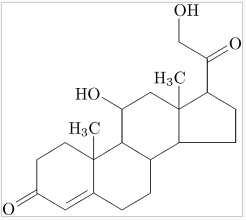
You can find the referenced image, chemicals.png at ../files/chemicals.png.
Placing Images
LaTeX often places images a long way from the surrounding text, especially in big documents. This can even be several pages away from where they are being discussed. We can override the placement by adding a [h] or [ht] to the end of the \begin{figure} command, the h means that you definitely want the image here, t means the top of the page. You can also add an exclamation mark (!) to tell LaTeX to override some of its rules on placing images.
\documentclass{article}
\usepackage{graphicx}
\begin{document}
\begin{figure}[ht!]
\includegraphics{chemicals.png}
\end{figure}
\end{document}
Captioning Images
Like with tables we can caption an image using the \caption{} command and label it using the \label{} command, so that we can reference it elsewhere in the document. By convention labels for images start with the name “fig:”.
\documentclass{article}
\usepackage{graphicx}
\begin{document}
\begin{figure}[ht!]
\includegraphics{chemicals.png}
\caption{label{fig:chemicals}Corticosterone}
\end{figure}
\end{document}
Figure \ref{fig:chemicals} shows the chemical structure of Corticosterone.
Sizing Images
Image sizes on the page can be specified with the [width=xcm] or [height=xcm] options on the \includegraphics line. You can also specify this in inches by using in, or millimetres by using mm instead of cm.
\documentclass{article}
\usepackage{graphicx}
\begin{document}
\begin{figure}[ht!]
\includegraphics[width=12cm]{chemicals.png}
\caption{label{fig:chemicals}Corticosterone}
\end{figure}
\end{document}
Figure \ref{fig:chemicals} shows the chemical structure of Corticosterone.
Images Exercise
Place the following lines of code in the correct order:
- \includegraphics[width=5cm]{mypicture.jpg}
- \begin{figure}
- \end{figure}
- \caption{label{fig:mypic}A Picture of me}
Solution
2,1,4,3
Key Points
Images are inserted with the figure environment.
Tables are created with the tablular environment.
Locations can be specified with the [h] option meaning here, of [ht] meaning here, top.
Tables and images can have labels to make their referencing easier.
Tables and images can have captions.
Mathematical Equations and Computer Code
Overview
Teaching: 15 min
Exercises: 5 minQuestions
How do you add equations to your LaTeX document?
How do you add computer code to your LaTeX document?
Objectives
Understand how to insert equations and computer code into documents
Inline Equations
Inline equations appear in the normal text and start with a $ symbol and then writes out the equation text followed by another $, powers are specified with the ^ symbol, fractions using the \frac command and the sigma symbol can be brought in using \sum. For example writing $E=mc^2$ will display
or a more complex is
$x = \sum \frac{e^\pi}{y^2-a}$.
\documentclass{article}
\begin{document}
	Einstein's famous formula $E=mc^2$....
\end{document}
\documentclass{article}
\begin{document}
	$x = \sum \frac{e^\pi}{y^2-a}$ is `$x = \sum \frac{e^\pi}{y^2-a}$
\end{document}
Labelled Equations
Sometimes we want an equation to be displayed on its own, especially when its a key part of a paper. For this we can use the equation environment with the \begin{equation} and \end{equation} commands. Like with tables and figures, these can also be labelled and then referenced elsewhere in the text.
\documentclass{article}
\begin{document}
\begin{equation}
E=mc^2
\label{eq:einstein}
\end{equation}
Einstein's famous equation is shown in equation \ref{eq:einstein}.
\end{document}
Useful Mathematical Symbols
This isn’t a complete list, see The Comprehensive LaTeX Symbol List for one.
\alpha\beta\delta\gamma\rho\sigma\epsilon\chi\tau\omega\lambda\theta
Computer Code
There are a few ways to include computer code in LaTex. The simplest in the verbatim environment which just shows the code inserted between the \begin{verbatim} and \end{verbatim} commands as it is, disabling any attempt to interpret it as LaTeX. It is usually shown in a courier font to differentiate it from other text, but otherwise has no styling.
\begin{verbatim}
#include<stdio.h>

int main(int argc,char **argv) {
  printf("Hello World\n");
  return 0;
}
\end{verbatim}
Computer programmers often like to use colours or different text styles to highlight the syntax of their code, for this the more elaborate listings package can do this. The example below will do a simple black and white version with keywords put into bold. For a more elaborate version using colour see this example from wikibooks.
\documentclass{article}
\usepackage{listings}
\begin{document}
\lstset{language=C}
\begin{lstlisting}
#include<stdio.h>

int main(int argc,char **argv) {
  printf("Hello World\n");
  return 0;
}
\end{lstlisting}
\end{document}
Captioning Code Listings
The listings package doesn’t support the \caption{} command we’ve used on tables and images. Instead add a caption parameter in [ and ] to the \begin{lstlisting} command. For example:
\begin{lstlisting}[caption=Caption text here]
Loading computer code from a file
Computer code can be loaded from a source file instead of being pasted into LaTeX. This way the document can always reflect the latest version of your code. This is done using the \lstinputlisting{} command, where the filename is the argument. An optional extra argument can specify the language inside square brackets [ and ] symbols with the word language= followed by the language name, for example [language=C] or [language=python].
\documentclass{article}
\usepackage{listings}
\begin{document}
\lstinputlisting[language=C]{helloworld.c}
\end{document}
Including and Equations Code Exercise
Create a LaTeX document with the following source code included. You can download this code as a file from ../files/sine_curve.py. Write a caption stating that this is the code for generating the curve of
import matplotlib as mpl
import matplotlib.pyplot as plt
import numpy as np
x = np.arange(0, 10, 0.1);
y = np.sin(x)
plt.plot(x, y)
plt.title('Sine Curve')
plt.show()
Solution
\documentclass{article}
\usepackage{listings}
\begin{document}
\lstset{language=python}
\begin{lstlisting}[caption={Below the code to generate the curve of $y=sin(x)$}]
import matplotlib as mpl
import matplotlib.pyplot as plt
import numpy as np
x = np.arange(0, 10, 0.1);
y = np.sin(x)
plt.plot(x, y)
plt.title('Sine Curve')
plt.show()
\end{lstlisting}
\end{document}
Key Points
Equations can be entered inline by starting and ending with a $
Equations can be placed on their own with the \begin{equation} command
There are lots of specialist symbols like greek letters available as their own commands
Computer code can be included with the verbatim or listings environments
Bibliographies
Overview
Teaching: 10 min
Exercises: 5 minQuestions
How do you include bibliographic references?
Objectives
Understand how to include bibliographic references in LaTeX
LaTeX lets you cite references as you go in your document and then produces a bibliography of all the references that were used. References are placed in an external file called a BibTeX database, where each reference will have a key to uniquely identify it. These keys can be anything you like, but typically they are the author’s name and the year or the title of the item. LaTeX then uses the \cite{} command to include a link to the reference.
Here is some example BibTex for a book about LaTeX and an article. goossens93 and greenwade93 are the keys which we’ll use to cite them inside LaTeX.
@book{goossens93,
    author    = "Michel Goossens and Frank Mittelbach and Alexander Samarin",
    title     = "The LaTeX Companion",
    year      = "1993",
    publisher = "Addison-Wesley",
    address   = "Reading, Massachusetts"
}

@article{greenwade93,
    author  = "George D. Greenwade",
    title   = "The {C}omprehensive {T}ex {A}rchive {N}etwork ({CTAN})",
    year    = "1993",
    journal = "TUGBoat",
    volume  = "14",
    number  = "3",
    pages   = "342--351"
}
The LaTeX code to reference these will be \cite{goossens93} or \cite{greenwade93}, the LaTeX compiler will replace these lines with a number or an author/date style reference inside the main text and then include them in bibliography. We also have to tell LaTeX what BibTex file to use with the \bibliography{} command, this takes the argument of the name of the bibliography without the .bib extension that is normally given to BibTeX files. We can also set the style of the bibliography with the \bibliographystyle{} command, common styles include the plain style which uses numbered references in the document and sorts the bibliography by author, the unsrt style does the same but sorts by the order of referencing and the named style uses the authors name and date instead of a number inside the text.
\documentclass{article}
\begin{document}
We can cite a text like \cite{goossens93}  or \cite{greenwade93} with the cite command.
\bibliography{library}
\bibliographystyle{unsrt}
\end{document}
Bibliographies exercise
Change the citation style in the text above to unsrt Some publishers will export bibtex from their websites that you can include in your database. Find the BibTeX for the paper “Soft Hair on Black Holes” by Stephen Hawking and add it to your database. Cite Hawking’s Paper in your text
Solutions
Hawking’s paper’s Bibtex can be found at https://journals.aps.org/prl/export/10.1103/PhysRevLett.116.231301 The code to cite it will be \cite{PhysRevLett.116.231301} (assuming you didn’t change the key’s name)
Key Points
LaTeX needs bibliography information to be stored in a separate BibTeX database.
Each bibtex entry needs a unique key
We cite bibtex entries with the \cite{} command
We make LaTeX display the bibliography with the \bibliography{} command, this also specifies the name of the bibtex database
We can choose the style of the bibliography with the \bibliographystyle{} command. Common ones are unsrt, plain or named
Many journals will offer you the option to download the BibTeX for a paper
Common Problems and useful tips
Overview
Teaching: 5 min
Exercises: 0 minQuestions
How do I format URLs into my document?
How do I insert some common symbols?
How do I get images into the right place?
Is LaTeX really worth all this hassle?
Are there any easier to use alternatives?
How do I convert LaTeX to MS Word for my colleague/journal who insists we use Word?
Objectives
Understand some common problems encountered in LaTeX and solutions to them
Know about some utilities to make LaTeX easier to use
URL Formatting
LaTeX often doesn’t like URLs in the code. Use the hyperref package and the \url{} command to include them, this will also make them a clickable hyperlink in the PDF. Sometimes certain characters have to be escaped with \ character in front of them. Alternatively you can change them to an ASCII code with the code \%<code>, using a code from asciitable.com. For example http://www.mysite.com/somepage?a=1&b=2 would become either \url{http://www.mysite.com/somepage\?a=1\&b=2} or \url{http://www.mysite.com/somepage\%3Fa=1\%26b=2.
Special Characters
- £ sign, use
\poundsor\textsterling <or>symbols:\textlessor\textgreater- Exponents (e.g. 2 8 ):
2\textsuperscript{8} - Degrees symbol (e.g. 45 ◦ ), load the siunitx package and use
$\SI{45}{\degree}$
Images in the wrong place
- Use [ht!] on the begin figure line:
\begin{figure}[ht!] - Move the source location of the image, this can make reading the source annoying but can make it appear in a better place on the page.
- Resize the image slightly by adjusting the
[width=xcm]or[height=xcm]to the\includegraphicscommand.
Is it worth the hassle?
- LaTeX might be more effort for smaller documents but it really pays off with bigger documents.
- Many Journals offer a LaTeX template and an example file which takes away a lot of the hard work.
Useful Utilities
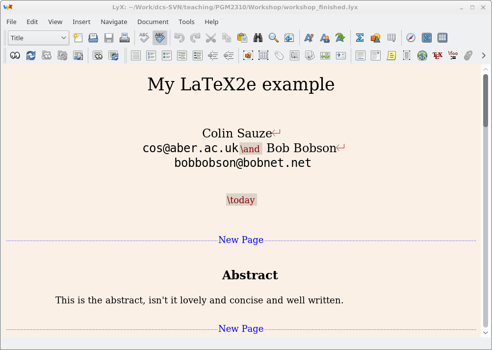
- LyX is a “What you see is what you mean” editor, it shows things in a nice graphical format that represent’s how you intend it to look but is nothing like how it will really look on paper. It can use LaTeX commands, import/export LaTeX files and produces documents by converting to LaTeX first.
-
latex2rtf converts LaTeX output to RTF files which can be read by MS Word. Useful for when you need to give somebody who doesn’t know LaTeX a document for them to edit or a Journal insists on Word file submissions.
-
jabref is a BibTeX database manager that lets you manage your BibTeX database. Mendeley can also export to BibTeX.
Key Points
Use the hyperref package and url command to handle URLs. Some characters might need escaping.
LaTeX has lots of commands for common special characters you might type in on the keyboard.
Images often appear in the wrong place, use [ht!], resize the image or move the reference to the image to a different place in the LaTeX code.
LaTeX can be hassle especially on smaller documents but really comes into its own on big documents.